 Open your "checks" workbook if it isn't already opened.
You will learn how to format a Google Spreadsheets workbook in this part of the tutorial.
Open your "checks" workbook if it isn't already opened.
Select the first row of the "checks" workbook, by clicking on the row header "1".
Observe: 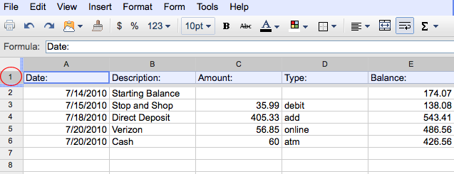
You have just selected what Spreadsheets describes as a range.
A range is a rectangular block of cells. Many things are accomplished in Spreadsheets using ranges. For instance, the format used to display values can be changed for an entire range. All the values in a range can be referred to when writing a formula. A range of cells can also be protected, which means the contents of the cells cannot be altered. Ranges can also be named.
With the range of cells A1:E1 selected, click on the Bold button and Center alignment button (as demonstrated below).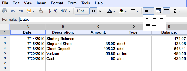
With the range of cells A2:A6 selected, click on the Center alignment button. Do the same for cells D3:D6.
If the formatting made the text too big for the cells, adjust the widths of the columns accordingly.
Observe: 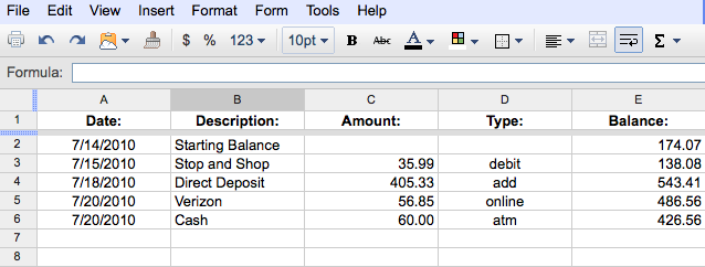
The basic formatting rule "select and then do" is used when working with Spreadsheets.
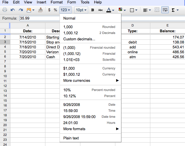
Google Spreadsheets automatically formats numbers and dates each time they are used. You can change the way certain values are formatted by selecting the  button for more formats. A menu will appear that lists the numerous ways for numbers and dates to be formatted, as shown below:
Select column C and format the dollar amounts by selecting the Currency option under the .
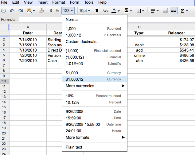
Next, with the range of cells C3:C6 selected, select the  (Format as currency) button to add a $ in front of the values.
Repeat for cells E2:E6.
Your "checks" workbook should look as follows: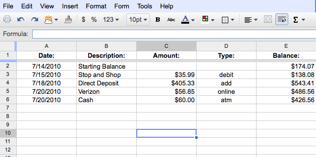
Let's insert a row between row 2 and row 3 in the "checks" workbook, to make the workbook more appealing to the eye.
Select row 3 by clicking on the row header "3".
Right click on row header "3" and choose Insert 1 above from the menu.
Now let's use some color and borders to format the workbook.
Select cells A1:E1. From the Toolbar, choose a fill color from the fill options (as shown below).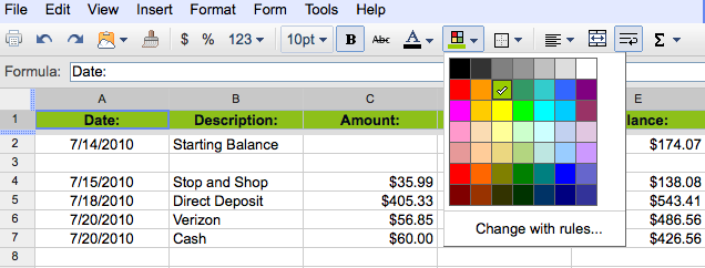
With cells A1:E1 still selected, choose "Bottom Border" from the borders menu (as shown below).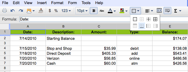
Finally, select cells B5:D5, choose a font color from the font colors menu (as shown below) to indicate that this entry is a deposit to the account.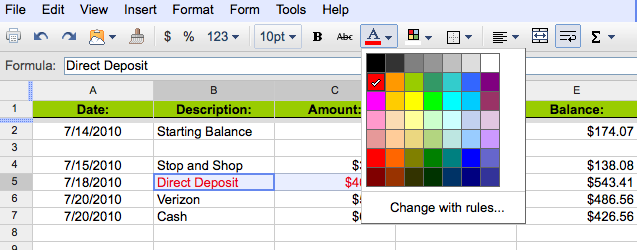
You have now learned how to format a Google Spreadsheets document and have completed your first workbook. Now it's time to preview your workbook.
Since changes are saved automatically, you can simply just close the workbook.
You are now ready to learn some advanced features of Google Spreadsheets.
Next Topic: Advanced Spreadsheets (Copying Cells)
Back to Main Menu